11.11 Summary
1. Key Review
- Bubble sort achieves sorting by swapping adjacent elements. By adding a flag to enable early return, we can optimize the best-case time complexity of bubble sort to \(O(n)\).
- In each round, insertion sort inserts an element from the unsorted portion into its correct position in the sorted portion. Although insertion sort has a time complexity of \(O(n^2)\), it remains very popular for small sorting tasks because each operation is relatively lightweight.
- Quick sort relies on sentinel partitioning. In sentinel partitioning, repeatedly choosing the worst possible pivot can degrade the time complexity to \(O(n^2)\). Choosing a median-based pivot or a random pivot can reduce the probability of this degradation. By recursing on the shorter subarray first, we can effectively reduce the recursion depth and optimize the space complexity to \(O(\log n)\).
- Merge sort includes two phases: divide and merge, which typically embody the divide-and-conquer strategy. In merge sort, sorting an array requires creating auxiliary arrays, with a space complexity of \(O(n)\); however, the space complexity of sorting a linked list can be optimized to \(O(1)\).
- Bucket sort consists of three steps: distributing data into buckets, sorting within buckets, and merging results. It also embodies the divide-and-conquer strategy and is suitable for very large data volumes. The key to bucket sort is distributing data evenly.
- Counting sort is a special case of bucket sort, which achieves sorting by counting the number of occurrences of data. Counting sort is suitable for situations where the data volume is large but the data range is limited, and requires that data can be converted to positive integers.
- Radix sort achieves data sorting by sorting digit by digit, requiring that data can be represented as fixed-digit numbers.
- Overall, we hope to find a sorting algorithm that is efficient, stable, in-place, and adaptive. However, as with other data structures and algorithms, no sorting algorithm can satisfy all of these criteria at the same time. In practice, we need to choose the appropriate sorting algorithm based on the characteristics of the data.
- Figure 11-19 compares mainstream sorting algorithms in terms of efficiency, stability, in-place property, and adaptability.
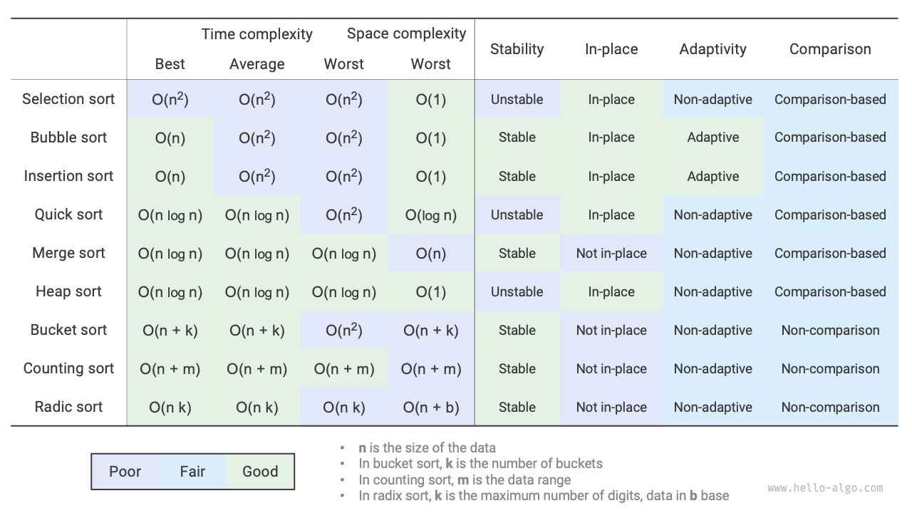
Figure 11-19 Sorting algorithm comparison
2. Q & A
Q: In what situations is the stability of sorting algorithms necessary?
In reality, we may sort based on a certain attribute of objects. For example, students have two attributes: name and height. We want to implement multi-level sorting: first sort by name to get (A, 180) (B, 185) (C, 170) (D, 170); then sort by height. Because the sorting algorithm is unstable, we may get (D, 170) (C, 170) (A, 180) (B, 185).
We can see that students D and C have swapped positions, destroying the ordering by name, which is not what we want.
Q: Can the order of "searching from right to left" and "searching from left to right" in sentinel partitioning be swapped?
No. When we use the leftmost element as the pivot, we must first "search from right to left" and then "search from left to right". This conclusion is somewhat counterintuitive; let's analyze the reason.
The last step of sentinel partitioning partition() is to swap nums[left] and nums[i]. After the swap is complete, the elements to the left of the pivot are all <= the pivot, which requires that nums[left] >= nums[i] must hold before the last swap. Suppose we first "search from left to right", then if we cannot find an element larger than the pivot, we will exit the loop when i == j, at which point it may be that nums[j] == nums[i] > nums[left]. In other words, the last swap operation will swap an element larger than the pivot to the leftmost end of the array, causing sentinel partitioning to fail.
For example, given the array [0, 0, 0, 0, 1], if we first "search from left to right", the array after sentinel partitioning is [1, 0, 0, 0, 0], which is incorrect.
By the same reasoning, if we select nums[right] as the pivot, the order is reversed: we must first "search from left to right".
Q: Regarding the optimization of recursion depth in quick sort, why can selecting the shorter array ensure that the recursion depth does not exceed \(\log n\)?
Recursion depth is the number of recursive calls that have not yet returned. Each round of sentinel partitioning divides the original array into two sub-arrays. After this optimization, the sub-array selected for further recursion is at most half the length of the original array. In the worst case, if it is always half as long, the final recursion depth is \(\log n\).
Reviewing the original quick sort, we may continuously recurse on the longer array. In the worst case, it would be \(n\), \(n - 1\), \(\dots\), \(2\), \(1\), with a recursion depth of \(n\). Recursion depth optimization can avoid this situation.
Q: When all elements in the array are equal, is the time complexity of quick sort \(O(n^2)\)? How should this degenerate case be handled?
Yes. In this case, the array can be partitioned into three parts through sentinel partitioning: less than, equal to, and greater than the pivot. We then recurse only on the less-than and greater-than parts. With this approach, an array whose elements are all equal can be sorted in just one round of sentinel partitioning.
Q: Why is the worst-case time complexity of bucket sort \(O(n^2)\)?
In the worst case, all elements are distributed into the same bucket. If we use an \(O(n^2)\) algorithm to sort these elements, the time complexity will be \(O(n^2)\).